Kaggle 데이터셋 중 Technology Company Layoffs(2022-2023)
을 분석한 자료입니다.
이번 시간에는 캐글 데이터를 확인하던 중, 최근에 올라온 흥미로운 데이터셋이
있어 몇가지 확인해보고, 비지도학습을 넣어볼 예정입니다.
미래의 우리와 관련이 있을 수도 있는 Technology company의 근무자 중 layoff 상태가 된 인원의 분석입니다.
layoffs는 기업측의 사정으로 인해 일시적 해고를 의미합니다. 여기서는 '정리해고'나 '구조조정' 정도의
의미로 통할 수 있습니다.
안타깝게도 한국의 사례는 없고 미국과 캐나다, 일부 유럽의 사례를 조사한 데이터입니다.
현재 기준, 제출된지 하루 밖에 되지않은 따끈따끈한 통계자료입니다.
잦은 구조조정은 우리나라만의 문제는 아니었군요.
이 데이터의 목적은 IT기업의 사례와 산업의 트렌드를 어느정도 보는 것입니다.
진행하는 방향은 column 분석, KMEANS 클러스터링, 약간의 시각화로 이루어집니다.
✅ 언제나 그렇듯이 자료 분석상 오역과 자의적인 해석이 있을수 있으니 유의 바랍니다.
가능한한 코드로 표현하려 했으나, 지면 크기상 데이터프레임은 이미지화 했습니다.
먼저 데이터를 다운로드 받고, 몇가지 필요한 패키지들을 불러와줍니다.
# 필요한 패키지 load

import numpy as np
import pandas as pd
import matplotlib.pyplot as plt
import seaborn as sns

# 분류 종류

from sklearn.cluster import KMeans
from sklearn.decomposition import PCA
특별히 데이터를 Colab 내부 파일에 저장해두었고, pd를 통해 불러왔습니다. (단일 파일)
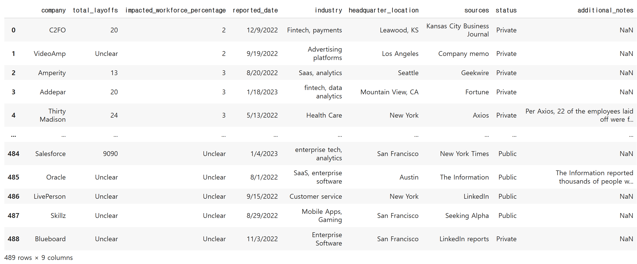
df = pd.read_csv('./tech_layoffs.csv')
df
train, test를 위한 목적은 딱히 없기 때문에 파일은 한 가지 입니다.
info로 정보를 확인합니다.
df.info()<class 'pandas.core.frame.DataFrame'>
RangeIndex: 489 entries, 0 to 488
Data columns (total 9 columns):
# Column Non-Null Count Dtype
--- ------ -------------- -----
0 company 489 non-null object
1 total_layoffs 489 non-null object
2 impacted_workforce_percentage 489 non-null object
3 reported_date 489 non-null object
4 industry 489 non-null object
5 headquarter_location 489 non-null object
6 sources 489 non-null object
7 status 489 non-null object
8 additional_notes 22 non-null object
dtypes: object(9)
memory usage: 34.5+ KB
수치형 데이터가 있는 것으로 보이는데, column이 전부 object 타입으로 되어있습니다.
Technology Company Layoffs (2022-2023)의 독특한 특징
바로 결측치를 넣는 대신 Unclear(불명확)이라는 문자열을 전부 채웠기 때문인데요?

추후 보게되는 데이터프레임입니다. 위에서처럼 total_layoffs 열만 해도 Unclear가 182개나 되는 것을 볼 수 있습니다.
다른 열에도 Unclear가 각계각층에 포진되어 있습니다.
기업의 대외비 사항인지, 통계청 내부의 사정때문인지 이처럼 data 원본에 결측치가 없다는 것이 특징입니다.
어떠한 측면에서는 불편하다고 볼수 있겠네요.
그리고 위 데이터셋을 볼때 생각해두어야 할 column들에 대한 설명입니다.
참고적으로 현재 kaggle 상에서는 회사에 따른 해고 인원, 산업군에 따른 해고 인원,
본사 위치에 따른 해고 인원, 공공/사기업에 따른 해고 인원 등 다양한 변수에 따른 해고 비율을
살펴보는 코드들이 눈에 띄고 있습니다.
아직까지는 미래 예측이나 비지도학습에 분류는 없는 것으로 보입니다.
(해당 분석들은 딱히 참조하지 않았습니다)
df.describe(include = 'O')
# df.describe()
# 결측치는 Unclear
다만 공통적으로 배제하는 것은 additional_notes 입니다. 일종의 '비고'처럼 쓰인 것으로 보이는데요.
이 열은 drop합니다.
# 불필요한 additional_notes 열 삭제
df.drop(['additional_notes'], axis = 1, inplace = True)
어떻게 분류를 해야할지 고려하던 중, 일단 회사를 기준으로 잡아보고자 했습니다.
layoff이니 회사를 중심으로 잡는 것도 적절한 접근으로 보였습니다.
df = df.sort_values(by='company')
df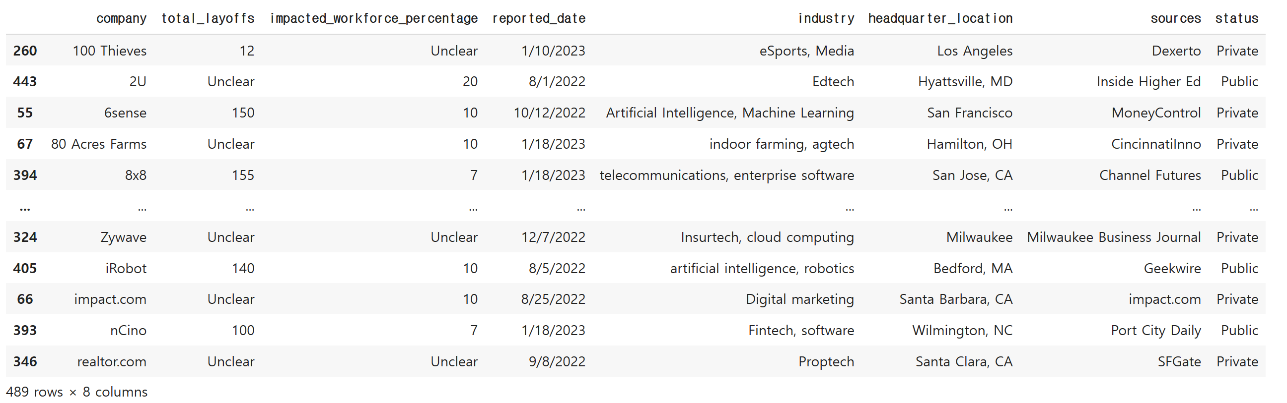
헌데 문제는 회사 수가 거의 행의 수에 근접할 정도로 많다는 점입니다.
len(df['company'].unique())477
회사명
df['company'].unique()array(['100 Thieves', '2U', '6sense', '80 Acres Farms', '8x8', '98point6',
'Abra', 'Addepar', 'Adobe', 'Advata', 'Adwerx', 'Affirm', 'Ahead',
'Airtable', 'Akili Interactive Labs', 'Albert', 'Almanac',
'Alphabet', 'Alto Pharmacy', 'Amazon', 'Amdocs', 'Amobee',
'Amount', 'Amperity', 'Apartment List', 'Apollo', 'AppLovin',
'Aqua Security', 'Arc', 'Argo AI', 'Argyle', 'Armis Security',
'Asana', 'Aspire', 'Assure', 'Astra', 'Astronomer', 'AtoB', 'Aura',
'Autobooks', 'Autograph', 'Automox', 'AvantStay', 'Baakt', 'Balto',
'Baton', 'Beachbody', 'Benitago Group', 'Better.com',
'Beyond Meat', 'BigBear.ai', 'BigCommerce', 'Bird', 'Bitfront',
'Bizzabo', 'BlackLine', 'Blend', 'BlockFi', 'BloomTech',
'Blue Apron', 'Blueboard', 'Bolt', 'Bonterra', 'Booking.com',
'Boosted Commerce', 'Brave Care', 'Brex', 'Bright Machines',
'Brightline', 'Built In', 'Butler Hospitality', 'BuzzFeed',
'Buzzer', 'C2FO', 'Callisto Media', 'Calm', 'Cameo',
'Candy Digital', 'Canoo', 'Capitolis', 'Capsule', 'Carbon Health',
'Career Karma', 'CareerArc', 'Cart.com', 'Carta', 'Carvana',
'Cedar', 'Celsius', 'Cerebral', 'Change.org', 'Chargebee',
'Chili Piper', 'Chime', 'Chipper Cash', 'ChowNow', 'CircleCI',
'Cisco', 'Citizen', 'Citrix Systems', 'Clarify Health',
'Clear Capital', 'Clever Real Estate', 'ClickUp', 'Clubhouse',
'Clyde', 'CoSchedule', 'Code42', 'CoinDCX', 'Coinbase', 'Colossus',
중략
정말 많았는데요. 때문에 다른 항목을 찾아야 했습니다.
일단 날짜 데이터부터 object가 아닌 datetime 타입으로 바꾸고자 했습니다.
df['reported_date'] = pd.to_datetime(df['reported_date'])
df.info()
<class 'pandas.core.frame.DataFrame'>
Int64Index: 489 entries, 260 to 346
Data columns (total 8 columns):
# Column Non-Null Count Dtype
--- ------ -------------- -----
0 company 489 non-null object
1 total_layoffs 489 non-null object
2 impacted_workforce_percentage 489 non-null object
3 reported_date 489 non-null datetime64[ns]
4 industry 489 non-null object
5 headquarter_location 489 non-null object
6 sources 489 non-null object
7 status 489 non-null object
dtypes: datetime64[ns](1), object(7)
memory usage: 34.4+ KB
다음으로 본 열은 industry 부분입니다.
# industry 별로 어떻게 정리해고가 들어가고 있을지 분석
df.industry.value_counts()
Fintech 24
Health Care 17
PropTech 15
E-commerce 13
Cybersecurity 10
..
Health care, pharmaceuticals 1
ecommerce, retail 1
cybersecurity, cloud infrastructure 1
food and beverage 1
Fintech, software 1
Name: industry, Length: 289, dtype: int64
아무래도 산업군이 object종류가 비교적 적을 것으로 보았습니다.
그리고 industry는 잡았으니, 지역으로 잡는 것은 어떨까요?
왜냐하면, 직업이나 산업군은 끝없이 증가할 수 있지만 미국의 국토는 증가하는 것이 요원하고
역사상 이벤트가 없는 한 증가할 일이 없기 때문이었습니다.
df['headquarter_location'].unique()array(['Los Angeles', 'Hyattsville, MD', 'San Francisco', 'Hamilton, OH',
'San Jose, CA', 'Seattle', 'Mountain View', 'Mountain View, CA',
'Bellevue, WA', 'Durham, North Carolina', 'Santa Clara, CA',
'Boston', 'Chesterfield, MO', 'Redwood City, CA', 'Chicago',
'Palo Alto', 'Burlington, MA', 'Pittsburgh', 'New York',
'Salt Lake City', 'Alameda, CA', 'Cincinnati', 'Detroit',
'Santa Monica, CA', 'Boulder', 'Alpharetta, GA', 'St. Louis',
'Manhattan Beach, CA', 'Columbia, MD', 'Austin, TX',
'Santa Monica', 'Palo Alto, CA', 'Jersey City', 'Distributed',
'Grand Rapids, MI', 'Portland', 'Leawood, KS',
'Emeryville, California', 'Torrance, California', 'Tempe',
'Hoboken, New Jersey', 'Playa Visa, California',
'Fort Lauderdale, FL', 'Truckee, CA', 'San Diego', 'Bismarck, ND',
'Minneapolis', 'Mumbai, India', 'Massachusetts', 'Austin',
'New City, NY', 'New York City', 'Walnut Creek, CA',
'Framingham, MA', 'Pleasanton, CA', 'Burlington, Massachusetts',
'Stamford, CT', 'San Franicsco', 'San Francsico', 'Bend, Oregon',
'Tempe, AZ', 'San Mateo, CA', 'Newton, Massachusetts',
'Nebraska City, NE', 'Columbus', 'Dever', 'The Bronx, NY',
'Atlanta', 'Dallas', 'Reston, VA', 'Philadelphia',
'Healdsburg, CA', 'Miami, FL', 'Greenville, SC',
'South Jordan, Utah', 'London', 'McLean, Virginia', 'Culver City',
'Louisville, CO', 'Stockholm', 'San Jose', 'New York, NY',
'Houston', 'Dover, DE', 'Bend, OR', 'Menlo Park, CA',
'Saratoga, CA', 'Waterford, MI', 'Los Gatos', 'Bay Area, CA',
'Denver', 'Phoenix', 'Lehi, UT', 'Englewood Cliffs, NJ',
'Charlotte, NC', 'Miami', 'Nashville, TN', 'Napa, CA', 'Tel Aviv',
'Draper, UT', 'Williston, VT', 'Provo, UT', 'Sunnyvale, CA',
'Belmont, CA', 'Irvine, CA', 'Menlo Park', 'Boca Raton, FL',
'Los Gatos, CA', 'Ottawa, Canada', 'Venice, CA',
'Incline Village, NV', 'Reno', 'Stockholm, Sweden', 'Lincoln, NE',
'Washington, DC', 'Newark, DE', 'Newton, MA', 'Purchase, NY',
'Oakland', 'Greater New York area', 'Walpole, MA', 'Oakland, CA',
'San Mateo', 'Stamford', 'Hayward, CA', 'Hayward, California',
'San Carlos, CA', 'Cambridge, MA', 'Indianapolis', 'Long Beach',
'Milwaukee', 'Bedford, MA', 'Santa Barbara, CA', 'Wilmington, NC'],
dtype=object)
본사 지역도 value 수가 매우 적다고 보긴 어렵지만, 그래도 회사명 보다는 적은 편입니다.
(134개)
❗ 독특한 점은 북미지역에 한정된 줄 알았는데, 스웨덴 스톡홀름, 캐나다 오타와, 영국 런던 등
대도시 일부도 보입니다.
※ 중간에 분수화 하다가 소숫점이 너무 길어지면 불편해지기 때문에 소숫점 자리는 4개 정도로 지정해줍시다.
pd.options.display.float_format = "{:.4f}".format
직종별 데이터를 int로 만들기 위해서 dummy 데이터로 만들었습니다.
industry_class = pd.get_dummies(df, columns=['industry'])
industry_class
좋습니다. 열이 289개정도 생겨났습니다.
사고를 방지하기 위해 데이터프레임은 복사해둡니다.
df1 = df.copy()(추후에 사용하지 않을 수도 있습니다)
그리고 산업군, 총 정리해고 수 외의 데이터는 제외시켜줍니다.
# industry, total_layoffs 이외의 데이터 제외
industry_class.drop(['company', 'impacted_workforce_percentage', 'reported_date','sources','status'], axis = 1, inplace = True)
industry_class
이제 결측치가 문제가 되기 시작하는데요.
object를 int로 바꿀려면 바꿀수 밖에 없게 됩니다.
Unclear는 어떻게 바꿔줘야 할지, 평균값 혹은 최빈값, 1이나 0 중에 고려했습니다.
industry_class = industry_class.sort_values(by='total_layoffs')
하지만 본 회사별 layoff를 조사하게 된 목적상 숫자가 '0'인 회사가 존재할까요?
분명 정리해고(구조조정)가 실질적으로 발생했기 때문에 조사가 되었을 것입니다.
또한 layoff 수가 10~9090까지 특별히 중위값을 계측할 수 없는 수치로 되어 있습니다.
이 때문에 평균값을 넣는 것도 유의미하지 않아 보입니다. min과 max가 너무 동떨어진 상황이네요.
# 실제 본 데이터에는 정리해고가 '실제로' 발생한 회사를 대상으로 했기 때문에 최소값인 1로 지정
industry_class = industry_class.replace({'total_layoffs': 'Unclear'}, 1)
industry_class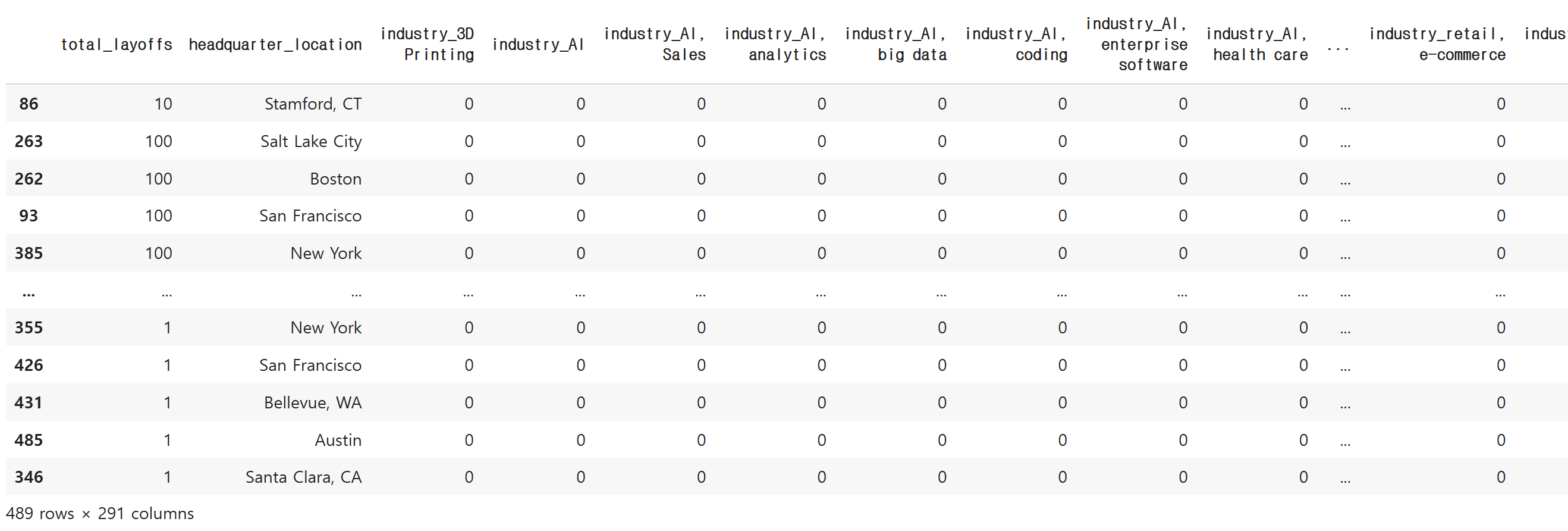
이번에는 Unclear 수치를 1로 설정했습니다. 적어도 그 상황(해고)이 한번은 발생했다고 본 것입니다.
드디어 dtype을 int로 바꿨습니다.
# total layoffs 타입을 int로 바꿈
industry_class = industry_class.astype({'total_layoffs':'int'})
industry_class
이제 다시 info로 타입들을 확인해보겠습니다.
industry_class.info(all)<class 'pandas.core.frame.DataFrame'>
Int64Index: 489 entries, 86 to 346
Data columns (total 291 columns):
# Column Dtype
--- ------ -----
0 total_layoffs int64
1 headquarter_location object
2 industry_3D Printing uint8
3 industry_AI uint8
4 industry_AI, Sales uint8
5 industry_AI, analytics uint8
6 industry_AI, big data uint8
7 industry_AI, coding uint8
8 industry_AI, enterprise software uint8
9 industry_AI, health care uint8
10 industry_AI, image recognition uint8
11 industry_AR, health care uint8
12 industry_Adtech, digital marketing uint8
13 industry_Advertising platforms uint8
14 industry_AgTech, food and beverage uint8
15 industry_Analytics uint8
16 industry_Artificial Intelligence uint8
17 industry_Artificial Intelligence, Machine Learning uint8
18 industry_Artificial intelligence, machine learning uint8
19 industry_Artificial intelligence, recruiting uint8
20 industry_Auto, E-commerce uint8
21 industry_Automotive, Ecommerce uint8
22 industry_Automotive, electric vehicles uint8
23 industry_Autonomous vehicles uint8
(중략)
열은 200개가 넘기때문에 생략했습니다.
일단 headquarter location 이외에는 모두 int형으로 바뀐것을 알 수 있습니다.
본사 위치는 사용할 것이기 때문에 object여도 문제 없습니다.
# 산업군, 본사 위치 제외 (label로 사용)
industry_class.iloc[:,2:]
이 for문이 관건입니다. 범주들의 이름으로 반복문을 돌리는데,
이제 기존에 있는 column에 새로운 값을 연산하는 것입니다.
특정 카테고리 X total layoffs을 하면 그 카테고리에 대한 정리해고 수가 들어갑니다.
아예 없다면 0만 반환되겠죠
# 특정 산업 포함여부 1/0로 치환
for col_name in industry_class.iloc[:,2:].columns:
    industry_class[col_name] = industry_class[col_name]*industry_class['total_layoffs']
그리고 본사 위치를 인덱스로 만들면서 & 카테고리별 해고 수를 합쳐줍니다.
(실제로는 이 데이터프레임에 열이 너무 많아서 눈에 잘 띄지 않습니다.)
# 회사의 본사 위치별로 정리해고된 크기 확인
industry_agg = industry_class.groupby('headquarter_location').sum()
industry_agg
기본적인 스케일링만 해줍니다.
robust scaling은 너무 나이브했고, min-max는 극단적으로 수치가 낮아져서 제외했습니다.
# 표준화 스케일링
from sklearn.preprocessing import StandardScaler

scaler = StandardScaler()
# 스케일링을 하고나서 데이터 조회
scaled = scaler.fit_transform(industry_agg)
scaled
array([[-0.24839921, -0.086711 , -0.086711 , ..., -0.086711 ,
-0.086711 , -0.086711 ],
[-0.24839921, -0.086711 , -0.086711 , ..., -0.086711 ,
-0.086711 , -0.086711 ],
[ 0.01990012, -0.086711 , -0.086711 , ..., -0.086711 ,
-0.086711 , -0.086711 ],
...,
[-0.24839921, -0.086711 , -0.086711 , ..., -0.086711 ,
-0.086711 , -0.086711 ],
[-0.23732043, -0.086711 , -0.086711 , ..., -0.086711 ,
-0.086711 , -0.086711 ],
[-0.22455574, -0.086711 , -0.086711 , ..., -0.086711 ,
-0.086711 , -0.086711 ]])
scaled_df로 표준화 스케일링한 headquarter_location별 해고자 수 데이터를 갖고 옵니다.
scaled_df = pd.DataFrame(scaled, columns=industry_agg.columns,
                         index=industry_agg.index)
scaled_df
현재 사용할 기법은 KMeans 클러스터링의 엘보우(elbow)기법 입니다.
군집을 몇개나 나누어야 군집화가 잘될지 판단하는 기법이었죠?
그래프에서 확실하게 꺾이는 지점을 찾아야 합니다.
# KMeans 표준화 - elbow
distance= []
for k in range(1, 21):
    k_model = KMeans(n_clusters = k, random_state = 10)
    k_model.fit(scaled_df)
    distance.append(k_model.inertia_)
일단 필자는 최초로 얼마나 꺾일지 알수 없어서 20개까지 cluster를 잡았습니다.
그래프 조회
sns.lineplot(x=range(1,21), y = distance)<matplotlib.axes._subplots.AxesSubplot at 0x7fb26ebb7af0>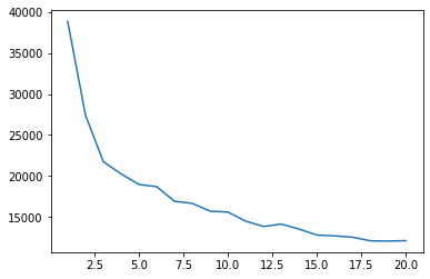
2~5사이에 꺾이는 지점이 보입니다.
# KMeans 표준화 - elbow
distance= []
for k in range(1, 8):
    k_model = KMeans(n_clusters = k, random_state = 10)
    k_model.fit(scaled_df)
    distance.append(k_model.inertia_)
sns.lineplot(x=range(1,8), y = distance)<matplotlib.axes._subplots.AxesSubplot at 0x7fb269a74f40>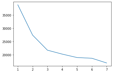
좋습니다. 2~3 정도가 적절한 cluster이겠네요.
k_model = KMeans(n_clusters=3, random_state=12)
labels = k_model.fit_predict(scaled_df)
k_model
KMeans(n_clusters=3, random_state=12)
결론적으로는 정리해고 합계가 높은 부분을 뽑아보려 했습니다.
미국에서 IT 종사자가 많은 지역이 영향이 있을까요? 새로 뜨는 지역이 영향을 끼칠까요?
scaled_df = scaled_df.sort_values(by='total_layoffs', ascending = False)
scaled_df
시각화 & Insight
scaled_df.head(10).iloc[:,:1].plot(kind = 'barh', color = 'green')
plt.title('City 10')
Text(0.5, 1.0, 'City 10')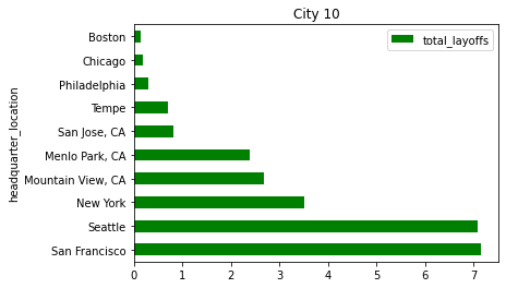
몇가지 범주를 더 보기 위해 20개 정도로 뽑아보겠습니다.
scaled_df.head(20).iloc[:,:1].plot(kind = 'barh')
plt.title('City 20')
Text(0.5, 1.0, 'City 20')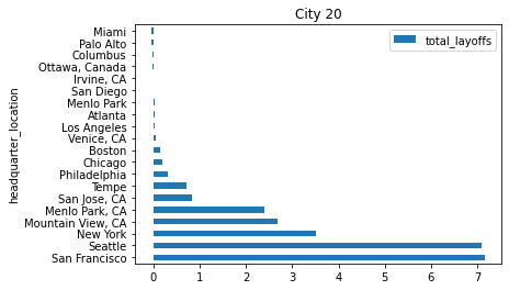
추가적인 인사이트가 있습니다. 바로 San francisco가 실리콘 밸리가 위치한 주 라는 것인데요.
아마존, 삼성전자 미국지사, 테슬라, 넷플릭스 등 공룡기업들이 즐비한 곳이죠.
존재 자체만으로도 구조조정 수에 영향을 미치는 것이 아닐까 싶습니다.
그 밑으로는 시애틀, 뉴욕, 캘리포니아의 몇몇 시가 위치하고 있습니다.
다만, 대단지 IT기업이 있는 LA나 텍사스가 눈에 띄진 않습니다.
💥 취업자 수가 아닌 Layoff 수치라는 점을 염두에 둬야 하겠습니다.
total layoff와 AI 산업간의 관계를 10개 지역정도로 추려서 보겠습니다.
plt.figure(figsize=(9,7))
sns.scatterplot(x='total_layoffs', y='industry_AI', data = scaled_df.head(10), hue = 'headquarter_location')

# 산점도의 각 카테고리 조합은 수십~수백개가 나올 수 있음
<matplotlib.axes._subplots.AxesSubplot at 0x7fb268ddab50>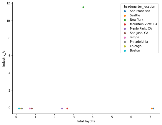
new york 부분에서 스케일링을 했는데도 특별히 큰 데이터가 발생한 것으로 보입니다.
scaling 전 데이터도 도시별로 확인해보겠습니다.
plt.figure(figsize=(9,7))
sns.scatterplot(x='total_layoffs', y='headquarter_location', data = industry_agg.head(20))
plt.title('total layoffs City 20')
# scaled 하기 전
Text(0.5, 1.0, 'total layoffs City 20')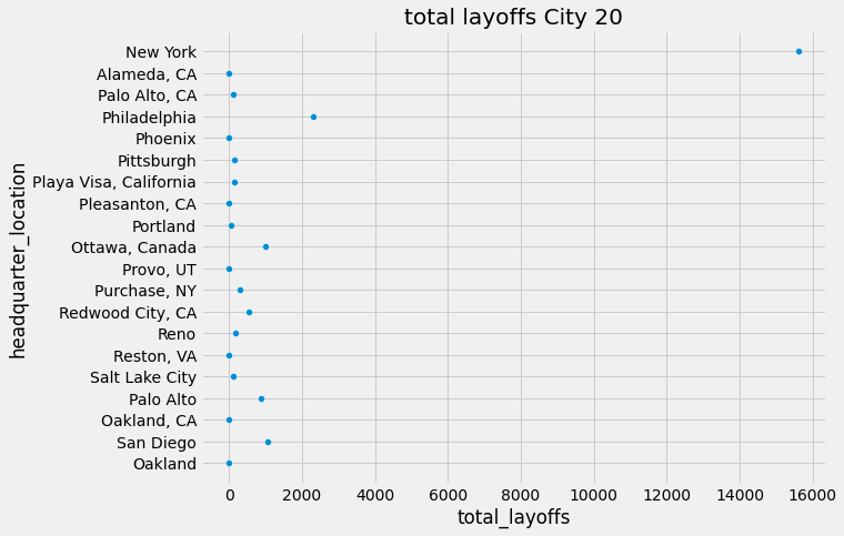
몇가지 스케일링과 지역구분을 바꿔야 할 필요성이 있겠네요.
column들을 추후에 다시 조정해보겠습니다.
'머신러닝 > 비지도학습' 카테고리의 다른 글
| [Machine Learning] PCA + Dimension 축소 학습 (1) | 2023.01.06 |
|---|
