
서론
이번 시간에는, 필자의 자유 주제로 kaggle에 분석용 데이터(Datasets)에
공유되어 있는 Video Game Sales를 활용해서, 여러가지 분석을
진행해보고자 합니다!
데이터셋 자체에 특별한 목표는 없지만, 일정한 흐름들은 있는데요.
바로 Global sales(전세계 판매량)과 그에 따른 platform이나, publisher(회사)의
순위들 입니다.
실제로 1100여건이 넘는 코드들을 보면 매우 다양한 방법으로 비디오 게임 데이터를
시각화한 그래프를 보실 수 있습니다.
아래는 원본 입니다.
https://www.kaggle.com/datasets/gregorut/videogamesales
Video Game Sales
Analyze sales data from more than 16,500 games.
www.kaggle.com
캐글에 업로드한 필자의 노트북도 공유합니다.
https://www.kaggle.com/code/apatheia0/video-game-lightgbm
개별적으로 필자가 제시한 목표는 global_sales에 영향을 준 변수들을 분석하고
어떠한 피쳐가 매출액에 영향을 주었는지 분석하는 것입니다.
※ 번역에 오류나 오판이 있을 수 있는점 양해 부탁드리며, 댓글 등으로 오류를 짚어 주시면 바로 수정하겠습니다.
※ 대부분 colab에서 데이터프레임을 표현할때는 원문을 가져왔으나, 데이터가 너무 큰 경우,
부득이하게 이미지로 캡쳐했습니다.
시작합니다
global_sales의 예측을 목표로, 다른 변수들의 중요도를 확인합니다
train모델은 GBM계열의 Classifier 알고리즘으로 학습할 예정입니다
필자는 colab상에서 원본 파일을 직접 업로드했습니다.
from google.colab import files
files.upload()
필요한 패키지나 라이브러리를 미리 불러왔습니다.
# 필요한 라이브러리 호출

import numpy as np
import pandas as pd
import seaborn as sns
import matplotlib.pyplot as plt
from sklearn.model_selection import train_test_split , RandomizedSearchCV
import xgboost as xgb
import lightgbm as lgb
파일을 호출합니다.
# 필요한 테스트 호출

df = pd.read_csv('/kaggle/input/videogamesales/vgsales.csv')
df
info를 통해 범주형 데이터들도 확인해봅니다.
df.info() # 더미데이터를 만들 object들 확인<class 'pandas.core.frame.DataFrame'>
RangeIndex: 16598 entries, 0 to 16597
Data columns (total 11 columns):
# Column Non-Null Count Dtype
--- ------ -------------- -----
0 Rank 16598 non-null int64
1 Name 16598 non-null object
2 Platform 16598 non-null object
3 Year 16327 non-null float64
4 Genre 16598 non-null object
5 Publisher 16540 non-null object
6 NA_Sales 16598 non-null float64
7 EU_Sales 16598 non-null float64
8 JP_Sales 16598 non-null float64
9 Other_Sales 16598 non-null float64
10 Global_Sales 16598 non-null float64
dtypes: float64(6), int64(1), object(4)
memory usage: 1.4+ MB
describe를 통해 최솟값과 최댓값을 확인해보고 데이터의 스케일링이
필요한지 고려해봅니다. 일단 점수를 높이기 위해 standard scaler를 써보겠습니다.
df.describe()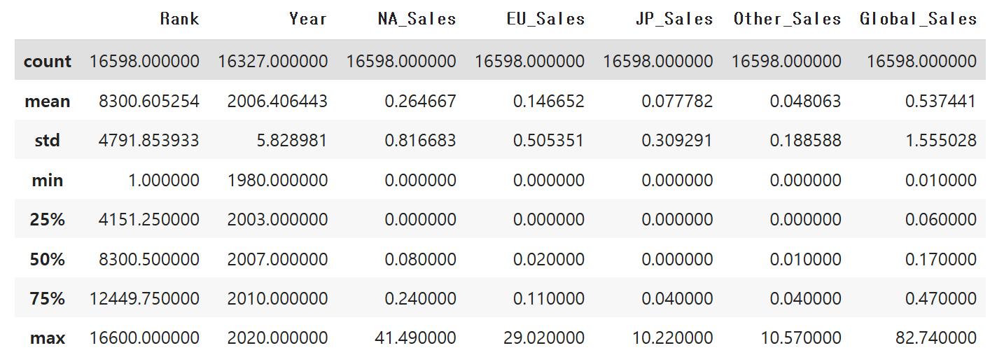
결측치를 확인하고 있습니다. Rank는 숫자폭이 크긴 한데, 추후에
삭제할 예정입니다.
# Name 열은 삭제예정
# 결측치 확인
df.isnull().mean()
# df.isnull().sum() # Year, Publisher 확인
Rank 0.000000
Name 0.000000
Platform 0.000000
Year 0.016327
Genre 0.000000
Publisher 0.003494
NA_Sales 0.000000
EU_Sales 0.000000
JP_Sales 0.000000
Other_Sales 0.000000
Global_Sales 0.000000
dtype: float64
Name과 Rank는 일단 전처리하기 전에 사용하는 곳이 없으므로 지웁니다.
항상 삭제에는 주의를 요합니다
# Name, Rank는 삭제
df2 = df.copy()
df = df.drop(['Name','Rank'], axis = 1)
이제 Year의 nan값을 어떻게 할지 고려합니다.
연도가 비어있는 곳은 어떻게 할까요.
# 결측치 처리 고려
df.Year.isna()
0 False
1 False
2 False
3 False
4 False
...
16593 False
16594 False
16595 False
16596 False
16597 False
Name: Year, Length: 16598, dtype: bool
TOP 20개 정도의 global sales 규모를 봤습니다.
df.Global_Sales.sort_values(ascending = False).head(20)0 82.74
1 40.24
2 35.82
3 33.00
4 31.37
5 30.26
6 30.01
7 29.02
8 28.62
9 28.31
10 24.76
11 23.42
12 23.10
13 22.72
14 22.00
15 21.82
16 21.40
17 20.81
18 20.61
19 20.22
Name: Global_Sales, dtype: float64
상관관계도 나타내봅니다.
year가 크게 변수에 영향을 미치는 점은 많지 않습니다.
sns.heatmap(df.corr(), annot=True, vmax = 1, vmin=-1)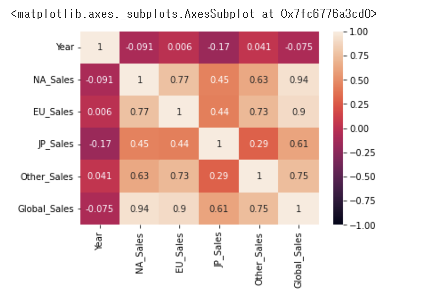
그러한 이유에서, 발매일 자체를 빈곳에서 없애는 것은
문제가 있어보입니다. 또한 전체에서 약 1.6%에 해당하는
비교적 영향력이 낮은 요소였습니다.
때문에 결측치 자체는 drop하도록 하겠습니다.
# 게임 발매일(Year)를 최빈값이나 평균값, 특정한 값으로 하는 것은
# 현실성이 없는 것으로 보임. dropna로 삭제
subset = ['year']

df = df.dropna(subset=['Year'])
df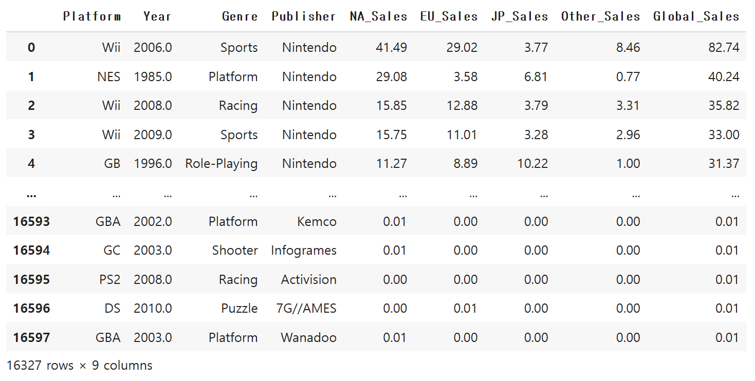
이제 publisher(배급사)의 결측치입니다.
# Publisher 결측치 고려
df.isna().sum()
Platform 0
Year 0
Genre 0
Publisher 36
NA_Sales 0
EU_Sales 0
JP_Sales 0
Other_Sales 0
Global_Sales 0
dtype: int64
조사기간 동안의 발매 숫자면에서 압도적인 1위 배급사는
Electronic Arts라는 곳입니다.
2위는 activision, 3위는 Bandai namco사가 자리잡고 있습니다.
언뜻 봐서는 Electronic Arts가 어떤 기업인지 몰랐었는데,
찾아보니 FIFA 시리즈로 유명한 EA 제작사 였더군요.
조사기간인 20세기 후반~2010년대까지는 니드포스피드 시리즈, 심즈 시리즈,
NBA시리즈, 각종 스튜디오 제품 등 굴지의 시리즈들을 보유하고 있네요.
최근에는 인디게임 제작에도 엄청난 투자를 하고 있다고 합니다.
추세를 봐서는 인디 분야에도 지원을 하니, 이 부분을 고려했습니다.
df.Publisher.value_counts() # 최빈값으로 채우기로 함Electronic Arts 1339
Activision 966
Namco Bandai Games 928
Ubisoft 918
Konami Digital Entertainment 823
...
Detn8 Games 1
Pow 1
Navarre Corp 1
MediaQuest 1
UIG Entertainment 1
Name: Publisher, Length: 576, dtype: int64
결측치는 해당 Publisher로 채우고자 합니다.
# Electronic Arts로 fill

df.Publisher = df.Publisher.fillna('Electronic Arts')
df.isnull().mean()
Platform 0.0
Year 0.0
Genre 0.0
Publisher 0.0
NA_Sales 0.0
EU_Sales 0.0
JP_Sales 0.0
Other_Sales 0.0
Global_Sales 0.0
dtype: float64
결측치는 모두 처리됬습니다.
이부분은 추후에 오류가 발생해서 추가해두었습니다.
df = df.astype({'Global_Sales': 'int'})
더미데이터 제작
# # 더미데이터 제작
# 두번째 세팅 시 , Publisher value가 너무 다양함
columns = ['Platform', 'Genre']

df = pd.get_dummies(df, columns = columns, drop_first = True)
df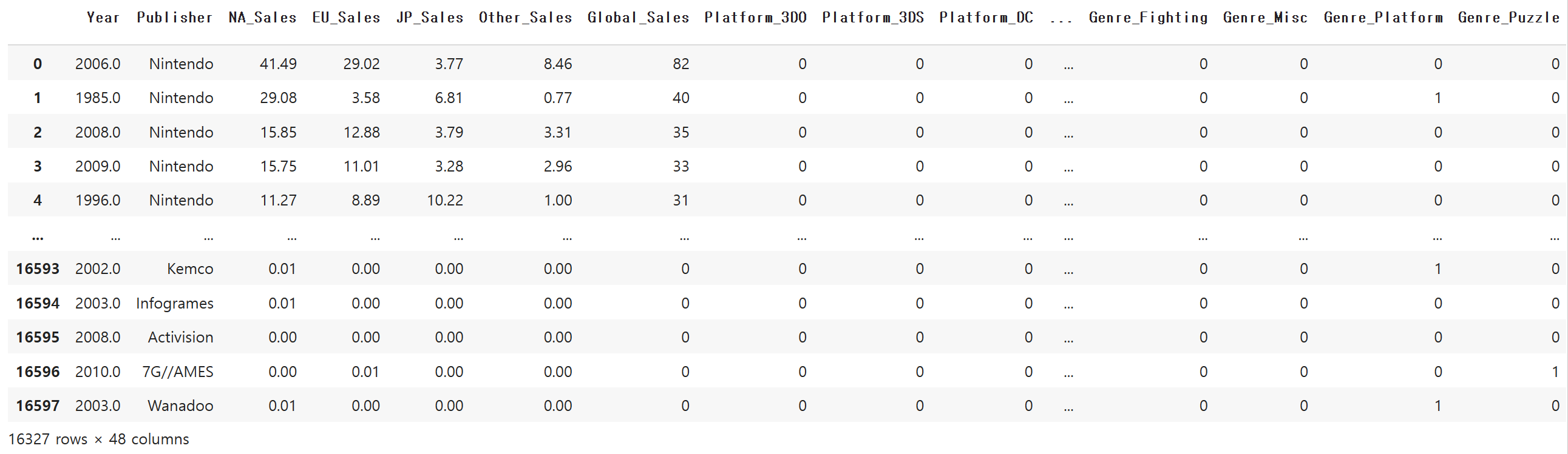
전처리는 이렇게 해서 종료되었습니다.
학습을 위해 훈련셋과 시험셋을 분리합니다.
# 전처리 종료
# 훈련셋, 시험셋 분리

# 과다한 시간 소요로 인해 Publisher는 삭제함
X = df.drop(['Global_Sales', 'Publisher'], axis = 1)
y = df['Global_Sales']

X_train, X_test, y_train, y_test = train_test_split(X, y, test_size=0.2, random_state=10)
초기 언급한것 처럼, 기초적으로 점수향상을 위해
스탠다드 스케일링은 진행했습니다.
from sklearn.preprocessing import StandardScaler
# 표준화 스케일링 시작

st_scaler = StandardScaler()
X_trainst = st_scaler.fit_transform(X_train)
X_testst = st_scaler.fit_transform(X_test)
분류 알고리즘은 최신의 LightGBM을 사용했습니다.
# LightGBM 분류기 정의
model = lgb.LGBMClassifier(random_state = 100)

model
LGBMClassifier(random_state=100)
FIT 진행
# lightgbm 학습 시작
model.fit(X_trainst, y_train)
pred = model.predict(X_test)
예측값도 조회홰봅니다만 이번 작업의 필수적인 코드는 아닙니다.
predarray([0, 0, 0, ..., 0, 0, 0])
정확도 점수를 뽑아봅니다.
# 정확도 점수 계산
from sklearn.metrics import accuracy_score
accuracy_score(y_test, pred) # 88점
0.8842620943049602
88점을 기록.
변수 중요도를 뽑아봤습니다.
# 변수 중요도 확인

feature_important = pd.DataFrame({
    'features' : X_train.columns,
    'values' : model.feature_importances_,
})
feature_important
	features	values
0	Year		3249
1	NA_Sales	11059
2	EU_Sales	7606
3	JP_Sales	5928
4	Other_Sales	4364
5	Platform_3DO	0
6	Platform_3DS	55
7	Platform_DC	1
8	Platform_DS	112
9	Platform_GB	78
10	Platform_GBA	26
11	Platform_GC	15
12	Platform_GEN	2
13	Platform_GG	0
14	Platform_N64	28
15	Platform_NES	56
16	Platform_NG	0
17	Platform_PC	51
18	Platform_PCFX	0
19	Platform_PS	46
20	Platform_PS2	106
21	Platform_PS3	65
22	Platform_PS4	52
23	Platform_PSP	70
24	Platform_PSV	8
25	Platform_SAT	11
26	Platform_SCD	0
27	Platform_SNES	33
28	Platform_TG16	0
29	Platform_WS	0
30	Platform_Wii	411
31	Platform_WiiU	2
32	Platform_X360	200
33	Platform_XB	351
34	Platform_XOne	8
35	Genre_Adventure	19
36	Genre_Fighting	40
37	Genre_Misc	117
38	Genre_Platform	107
39	Genre_Puzzle	26
40	Genre_Racing	167
41	Genre_Role-Playing	178
42	Genre_Shooter	52
43	Genre_Simulation	71
44	Genre_Sports	279
45	Genre_Strategy	43
sort_values로 내림차순 변환합니다.
	features	values
1	NA_Sales	11059
2	EU_Sales	7606
3	JP_Sales	5928
4	Other_Sales	4364
0	Year	3249
30	Platform_Wii	411
33	Platform_XB	351
44	Genre_Sports	279
32	Platform_X360	200
41	Genre_Role-Playing	178
40	Genre_Racing	167
37	Genre_Misc	117
8	Platform_DS	112
38	Genre_Platform	107
20	Platform_PS2	106
9	Platform_GB	78
43	Genre_Simulation	71
23	Platform_PSP	70
21	Platform_PS3	65
15	Platform_NES	56
6	Platform_3DS	55
22	Platform_PS4	52
42	Genre_Shooter	52
17	Platform_PC	51
19	Platform_PS	46
45	Genre_Strategy	43
36	Genre_Fighting	40
27	Platform_SNES	33
14	Platform_N64	28
39	Genre_Puzzle	26
10	Platform_GBA	26
35	Genre_Adventure	19
11	Platform_GC	15
25	Platform_SAT	11
34	Platform_XOne	8
24	Platform_PSV	8
12	Platform_GEN	2
31	Platform_WiiU	2
7	Platform_DC	1
5	Platform_3DO	0
16	Platform_NG	0
29	Platform_WS	0
28	Platform_TG16	0
13	Platform_GG	0
26	Platform_SCD	0
18	Platform_PCFX	0
이렇게 해서는 잘 보이진 않네요.
시각화로 그래프를 그려봅니다.
plt.figure(figsize=(12,9))
sns.barplot(x='values', y='features', data = feature_important.sort_values(by = 'values', ascending=False).head(20)
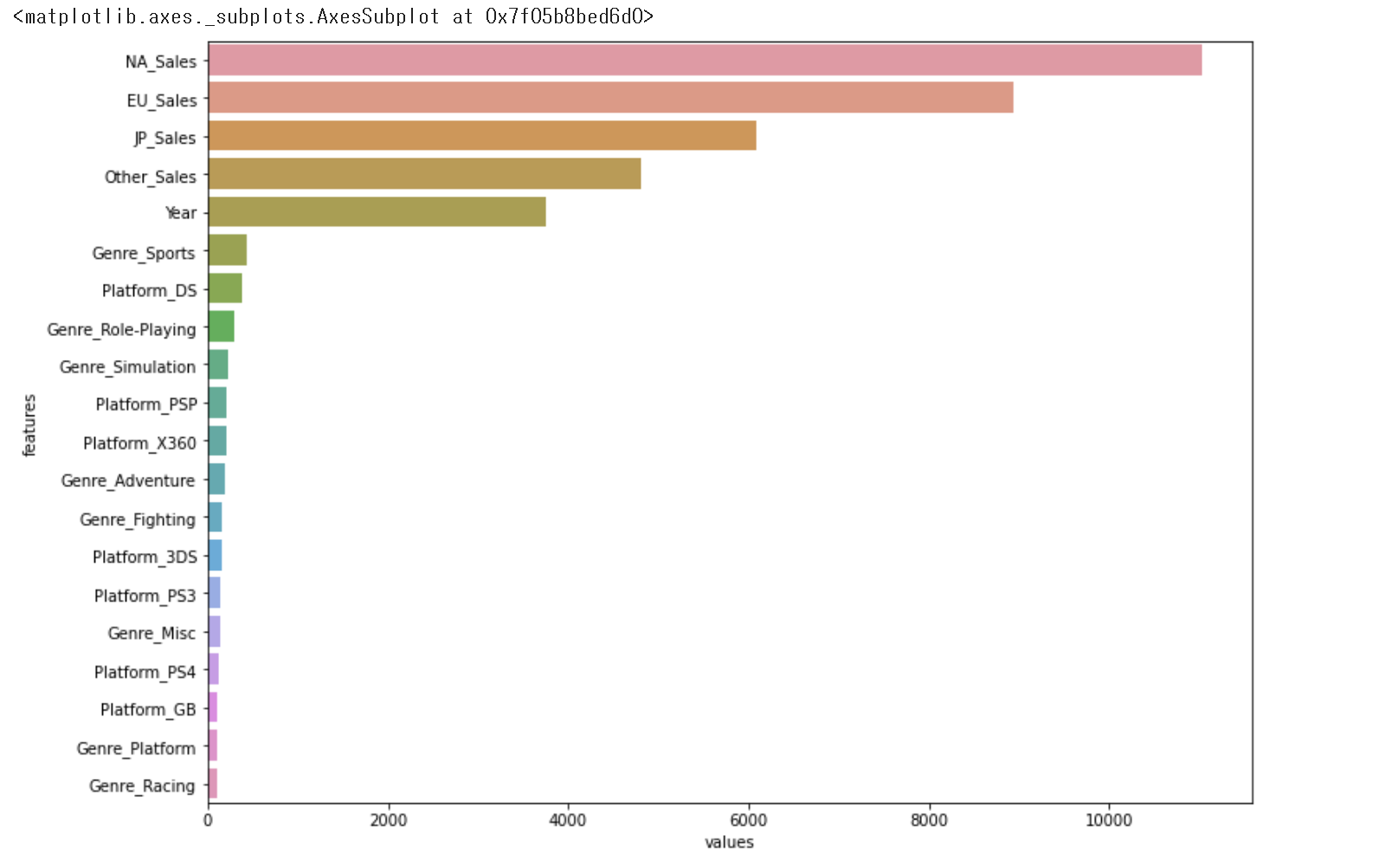
좋습니다만, 10위 이하부터는 수치가 미묘한 차이를 보입니다.
1~10위까지만 볼까요?
plt.figure(figsize=(12,9))
sns.barplot(x='values', y='features', data = feature_important.sort_values(by = 'values', ascending=False).head(10), palette = 'rainbow')
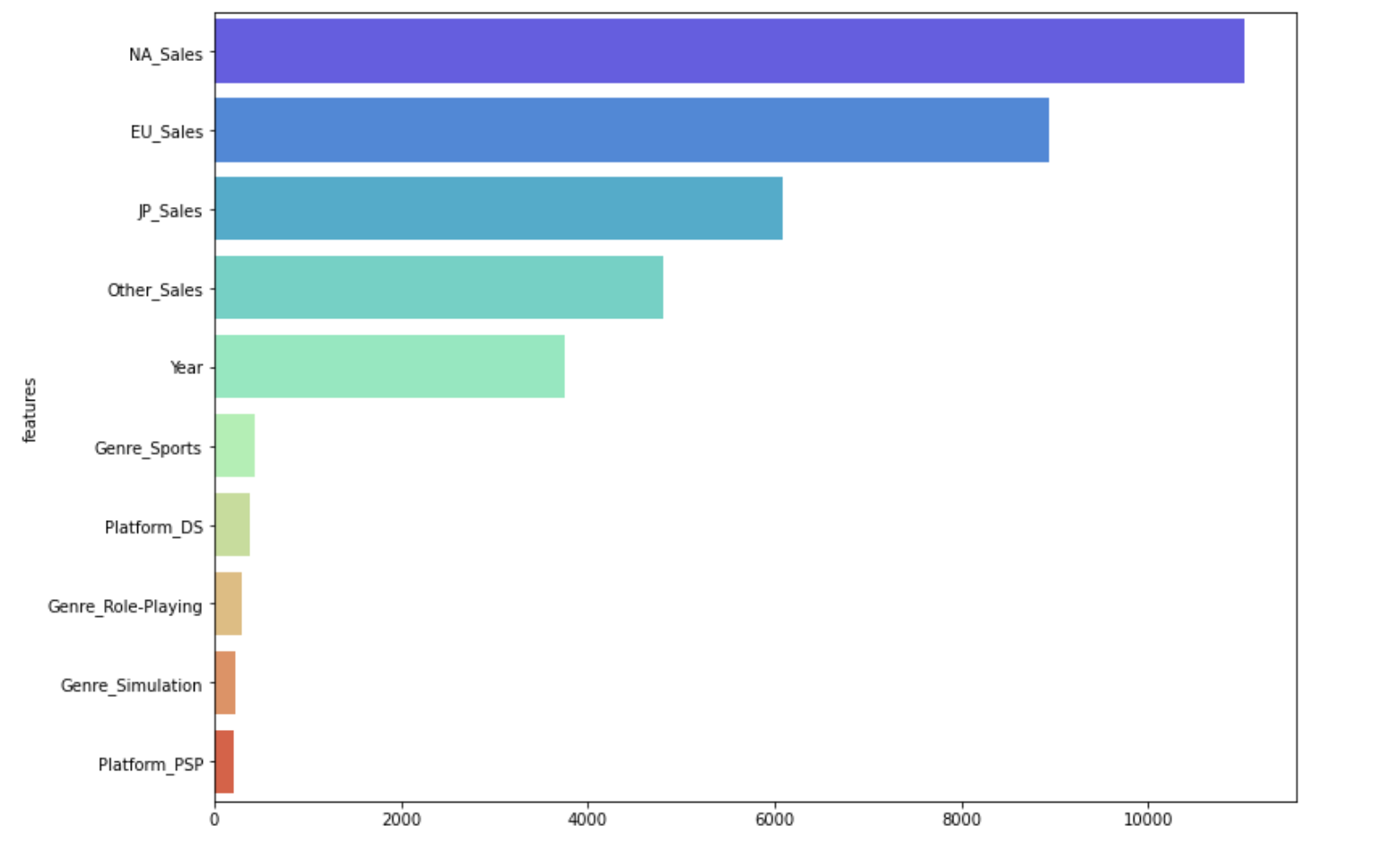
컬러감을 입히기 위해서, palette를 rainbow로 바꿨고, 10위권 까지 바꿨습니다.
1위는 NA sales (북미 지역 매출), 2위는 EU sales(유럽 매출), 3위는 JP sales(일본 매출)이
기록하고 있습니다. 장르면에서 스포츠가 영향을 준것도 인상 깊군요.
이렇게 해서, 시각화까지 완료했습니다!
'머신러닝 > 지도학습' 카테고리의 다른 글
| [Machine Learning] Kaggle_데이터셋 분석_미 초소형 기업 밀도 예측_ep.2 (0) | 2022.12.31 |
|---|---|
| [Machine Learning] Kaggle_데이터셋 분석_미 초소형 기업 밀도 예측 (0) | 2022.12.30 |
| [Machine Learning] Kaggle_연습사례 분석_Spaceship_titanic_2 (0) | 2022.12.28 |
| [Machine Learning] Kaggle_연습사례 분석_Spaceship_titanic (2) | 2022.12.27 |
| [Machine Learning] Naive_Bayes 모델_ep.2 colab 검색기 (0) | 2022.12.26 |


